• Facets (new session)
• Description
• Metadata
• Settings
  • Rule: ActivityStreamsMapasEquivalentb3sb3sifpdbprdf-labelfacetshttp://dbpedia.org/resource/inference/rules/dbpedia#http://dbpedia.org/resource/inference/rules/opencyc#http://dbpedia.org/resource/inference/rules/umbel#http://dbpedia.org/resource/inference/rules/yago#http://dbpedia.org/schema/property_rules#http://www.ontologyportal.org/inference/rules/SUMO#http://www.ontologyportal.org/inference/rules/WordNet#http://www.w3.org/2002/07/owl#ldpoplwebrel-me-authskos-transurn:det:rdf:labelurn:kidehen:glossary:inference:rulesurn:owl:inference:rules:testsvirtpivot-rulesvirtrdf-eturtle-containersvirtrdf-hashtagvirtrdf-ifpvirtrdf-labelvirtrdf-meta-entity-classvirtrdf-urlNone
    
  • Inverse Functional Properties: Disabled (fastest) Apply to subjects only Apply to objects only Apply to both subjects and objects
  • "Same As": Disabled (fastest) Apply to subjects only Apply to objects only Apply to both subjects and objects (recommended) Apply to subjects, objects and predicates (not recommended on big datasets) Apply to predicates only (special use cases only)

About: What Is the Capital Asset Pricing Model? CAPM Framework Explained     Goto   Sponge   NotDistinct   Permalink

An Entity of Type : schema:Thing, within Data Space : kingsley.idehen.net associated with source document(s)

Type: Thing New Facet based on Instances of this Class

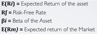
In finance, the capital asset pricing model (or CAPM) is a model or framework that helps theoretically assess the rate of return required for an asset to build a diversified portfolio able to give satisfactory returns.  CAPM assumptions The CAPM or Capital Asset Pricing Model, although unrealistic, it is still the most used in financial analysis. The reason I say unrealistic is that the CAPM even assumes that financial markets are perfect and investors rational.  Besides the debate about CAPM’s ability to predict reality, I am going to show you in detail how it works. In this section, I will use a sort of reverse engineering approach.  Almost like a Quentin Tarantino’s movie that starts from the end and slowly unravels until the beginning of the story, I will start from the CAPM formula and reverse engineer it backward: Don’t worry if it all looks nonsense right now. Just keep in mind that since returns are situated in the future, the purpose of this model is to compute the expected return of a security. Also, to do so, we will have to assess several factors. See below the meaning if the formula: Now we can break down the formula. The expected return of an asset is given by the risk-free rate + the Beta of the asset in which we invested multiplied by what is called the market risk premium (provided by the expected return of the market portfolio minus the risk-free rate).  Fine, what now? To compute the expected return of an asset we have to assess three variables: Risk-free rate Beta The expected return of the market Let me explain these variables further. What is the risk-free rate? In finance lingo, the risk-free rate is the % amount you will receive to invest in an asset that carries no risk. This means that you expected returns would be the same as your actual returns. Unless you are in Wonderland, there is no such thing as an asset that carries no risk at all. In fact, after the financial crisis of 2008, we understood how interconnected is the whole world economy and how a butterfly flap in Mexico can cause a tornado in China. This effect called butterfly effect, and it is used in chaos theory to explain how a tiny change in the initial state of a system can then have unpredictable consequences to its “final state.”  This happens, due to the complexity of the system. On the other hand, the risk-free rate will help us in determining the additional return we have to expect to decide whether that investment is worth undertaking. In fact, assuming investors are rational, they will ask for an additional return for each level of additional risk. In other words, the risk-free rate works like a baseline or starting point from which we build our model. Practically speaking what a risk-free rate is? For instance, the most known risk-free asset is the U.S. Treasury. In short, you buy a piece of the U.S. debt, and in exchange, they give you interests, plus the capital invested. What is the time value of money? What is the difference between a dollar today and a dollar tomorrow? You may argue that a dollar is a dollar and either you have it today or tomorrow is not going to make any difference.  Instead, the first principle that we learn in finance is that “A dollar today tomorrow” and this has nothing to do with inflation. In fact, assuming no inflation at all this principle still applies. Why? Just because when you have the money available, it can be invested or it can earn interests. In finance, this concept is called the time value of money.  In fact, until you are not receiving the money, you are not earning interests, and in turn, you are losing many opportunities. You may wonder how do you determine whether an amount of money today is better than in the future.  To solve the mystery, we will have to explore two new concepts: present and future value.  What is the present value? The present value tells you how much is worth today a sum of money that you will receive in the future. To compute the present value, we will have to take the amount of money we will receive in the future and divide it by (1 + r)^t. We will call r the discount rate and t the number of years corresponding to when the money will be received. For instance, let’ assume that you want to save money for your kids. In short, you want to create a fund so that you will be able to pay for their education.  Your target is to save $100k in 10 years. Assuming that the fund offers a 5% simple annual interest, how much do you have to invest today to have $100k in the future? Easy: PV = Money in the future / (1 + discount rate)^Number of years in the future= 100,000 / (1+5%)^10 = $61,391 This means that if we want to receive $100k in ten years, we will have to invest $61,391 today! What is the future value? Imagine now the opposite scenario. You have $100k today, how much will it be worth in the future? To compute the present value we took the future amount and divided it by (1+r)^t.  To compute the future value, we will have to take the present amount and multiply it by (1+r)^t. Thus, assuming you want to know how much will $100k worth in 10 years, how do you do that? Assuming a risk-free rate of 5% simple annual interest: FV = Money you have today * (1 + discount rate)^ number of years in the future = 100,000 * (1+5%)^10 = 162,889 For the principle that a dollar today is worth more than a dollar tomorrow, in ten years, at 5% simple annual interest, your $100K will be worth $162,889! Now we covered the time value of money and thus how present and future value work, we can move forward and find out what Beta is. What is the Beta in CAPM? Regression analysis determines how an independent variable influences a dependent variable. Statistically speaking this means that we will collect a bunch of data to see the existing relationship between our stock and the market portfolio.  In fact, the objective here is to determine to what extent the stock we are analyzing is more or less risky compared to the market portfolio.  Thus, once collected the data they will appear on a graph that has two axes (x, y) and in that set of data, we will fit a line.  The Beta gives the slope of that line. In short, the higher the Beta, the higher will be the slope of the line and vice versa. In statistics, this kind of regression is also called linear regression. Beta (CAPM) formula The formula to compute our Beta is given by: The covariance is a statistical measure that allows us to understand if two variables are positively or negatively correlated. For instance, a positive covariance means that two variables move in the same direction, and vice versa.  The variance instead is a statistical measure that shows how values move away from the mean. Thus, it shows how values are spread around the mean. In fact, when there are larger moves around the mean, this also makes the stock riskier. *Together with the variance another significant measure of risk is the standard deviation (σ), which is the square root of the variance. When for instance, you see two stocks, A and B, where A has a σ of 20%, while B has a σ of 5%, A will be riskier than B. Furthermore, if you expect the same return between A and B, let’s say 10%, you will be better off to pick B. Why so? For the same level of return, you have a lower level of risk. Going back to the Beta. Once we divide the covariance of the two variables (stock and market portfolio) and the variance of the market portfolio we will determine for each movement up or down of the market portfolio, what is the movement of the security we are analyzing. That's it! What to read next? What is a financial option?  What is risk in finance? What is a financial ratio?  13 financial ratios formulas